OhmPediaPassive Components and LawsKirchhoff's Circuit Laws
Kirchhoff's Circuit Laws
基尔霍夫定律 Σ I = 0 (node) · Σ V = 0 (loop)
- Symbol
- Σ I = 0 (node) · Σ V = 0 (loop)
- Unit
- currents in amperes · voltages in volts · signs follow a chosen convention
- Section
- Passive Components and Laws
- Published
- 2026-08-29
- Author
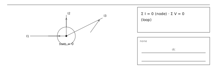
Kirchhoff's current law states that the algebraic sum of currents at any node is zero; the voltage law states that the algebraic sum of voltages around any closed loop is zero. Together they are sufficient to solve any linear resistive network, and they hold at every instant of time, not merely on average.
Charge and energy conservation applied to a circuit: currents into a node sum to zero, voltages around a loop sum to zero.
Sign convention does the work
Both laws are trivially true once you fix a convention and stick to it. The workable one is: assign every element a current arrow first, then write a voltage drop as positive when you traverse that element in the direction of its arrow. If the solved value comes out negative, the real current runs the other way — that is information, not an error. Most mistakes blamed on Kirchhoff's laws are actually sign errors introduced between the diagram and the equation.
Two laws solve every linear network
Nodal analysis writes the current law at each node and solves for node voltages; mesh analysis writes the voltage law around each independent loop and solves for loop currents. Either method alone is sufficient, and the choice is a matter of which produces fewer unknowns.
- Nodal analysis: one equation per node except the reference; unknowns are voltages. Best when there are many parallel branches and few loops.
- Mesh analysis: one equation per independent loop; unknowns are currents. Best for planar networks with few loops.
- Both methods scale as O(n³) in the number of unknowns, which is why circuit simulators use sparse matrix techniques instead.
Superposition and its limits
In a linear network the response to several sources is the sum of the responses to each source alone, with the others replaced by their internal impedance — a short for an ideal voltage source, an open for an ideal current source. Superposition simplifies hand analysis enormously but it does not apply to power, because power depends on the square of the current and squaring is not linear.
Three resistors meet at a node: 5 V through 1 kΩ, ground through 2 kΩ, and 3.3 V through 470 Ω. Writing the current law with the node voltage V as the unknown gives (5 − V)/1000 + (3.3 − V)/470 = V/2000. The left side evaluates to 0.005 + 0.00702, and the coefficients on V sum to 0.001 + 0.00213 + 0.0005 = 0.00363 per volt. Solving: V = 0.01202 / 0.00363 = 3.31 V. The same network solved by superposition gives three partial contributions of 3.60 V, 1.82 V and −2.11 V, which also sum to 3.31 V.
Read first
- Ohm's Law 欧姆定律
- Resistance 电阻
Adjacent entries
Off the shelf
Sources
- Physics LibreTexts https://phys.libretexts.org/Bookshelves/University_Physics/University_Physics_(OpenStax)/University_Physics_II_-_Thermodynamics_Electricity_and_Magnetism_(OpenStax)
- NDT Resource Center https://www.nde-ed.org/Physics/Electricity/ohmslaw.xhtml